
In magnetotellurics (or MT for short), we look at how electric and magnetic fields are induced within the Earth in order to understand how the Earth conducts electricity. The manner in which the Earth conducts electricity can tell us about many interesting physical processes and phenomena within the Earth. For example, as magma conducts electricity quite well, MT is useful for studying the movement and storage of magma at depth in the Earth. As another example, the electrical conductivity of Earth materials is at least partially controlled by temperature. MT is therefore also useful in detecting temperature anomalies deep within the Earth.
As you may remember from a physics class that you may have taken at some point, a time-varying electric field will generate a time-varying magnetic field, and vice versa. Here at the Earth's surface, we are surrounded by naturally occurring, time-varying electric and magnetic fields due to things like lightening strikes, electrical currents flowing in the ionosphere/magnetosphere, and solar (geomagnetic) storms. Those time-varying fields induce secondary fields within the Earth, and the manner in which those secondary fields are generated is controlled by how the Earth conducts electricity (which we call the conductivity structure of the Earth).
This process is illustrated in the animation below. A time-varying electric field at the Earth's surface induces electric and magnetic fields within the Earth. There are a few important things to take away from this animation. First, lower-frequency (long period) oscillations are able to penetrate deeper into the Earth than higher-frequency (short period) oscillations. Longer period variations in the electric and magnetic fields therefore tell us information about how the Earth conducts electricity at greater depths. Second, the relative magnitude of the electric and magnetic fields at the Earth's surface is controlled by the entire conductivity structure of the Earth at depth. The bottom plot has an added conductive layer at a depth of ~50 km, and you can see that this changes how the magnetic field (H) behaves. This is very important, as it means that by measuring the natural variations in the electric and magnetic fields at the Earth's surface, we're actually able to say something about how the Earth conducts electricity at depth. This is how MT works!
(A side note: the numbers shown on the layers in the animation are the resistivities of the layers. We often think in terms of this value, which is this inverse of conductivity. Lower values mean that electricity will flow better, and vice versa. Also, the physical laws of electromagnetism require that the electric and responding magnetic fields are orthogonal to each other in space. In the animation, I have plotted them both in the same plane simply to illustrate how they vary in time.)
So, in MT we go out and measure the electric and magnetic fields at the Earth's surface in order to understand the conductivity structure within the Earth. For the magnetic field, we use either three fluxgate magnetometers or three induction coil magnetometers to measure variations in the magnetic field in the three spatial dimensions. For the electric field, we simply measure the variations in the potential difference (the voltage difference) between two points on the Earth's surface and then calculate the electric field from that. We measure the potential difference in the two horizontal spatial dimensions at the Earth's surface. The images below give you an idea of what an MT site looks like. We place the electrodes to measure the potential difference ideally about 100 m apart and connect them to the recorder with long wires. We bury the magnetometers in order to isolate them from wind and thermal effects. (We are trying to make very precise measurements, so even the subtle movement of the magnetometers by gusts of wind can be problematic.)
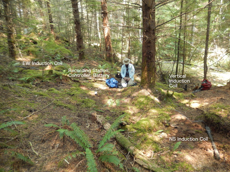 A Typical MT Site |
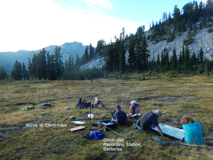 A More Scenic MT Site |
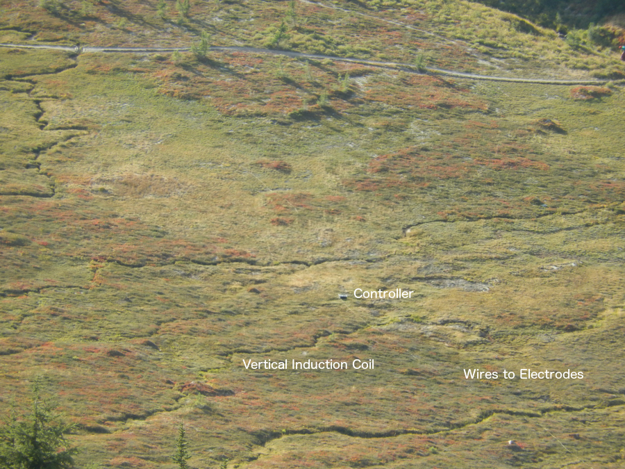 Looking Down at an MT Site |
We can derive the equations that describe electromagnetic induction in the Earth directly from Maxwell's Equations. For our purposes, Maxwell's Equations in differential form are as follows...
$$ \nabla \cdot \mathbf{E} = \frac{\rho}{\epsilon_0} $$ $$ \nabla \cdot \mathbf{H} = 0 $$ $$ \nabla \times \mathbf{E} = - \mu_0 \frac{\partial \mathbf{H}}{\partial t}$$ $$ \nabla \times \mathbf{H} = \mathbf{J} + \epsilon_0 \frac{\partial \mathbf{E}}{\partial t} = \sigma \mathbf{E} + \epsilon_0 \frac{\partial \mathbf{E}}{\partial t} $$
Here we are allowing for static source terms within the Earth (i.e., stationary free charges, so the divergence of \( \mathbf{E} \) does not necessarily vanish). Also, instead of writing the equations in terms of \( \mathbf{E} \) and \( \mathbf{B} \), which may be more familiar, I've used \( \mathbf{E} \) and \( \mathbf{H} \). Various texts call \( \mathbf{H} \) and \( \mathbf{B} \) different things and favor one over the other. I personally think that \( \mathbf{H} \) is more physical, since it stays the same regardless of whether you are in a dielectric or in free space (like \( \mathbf{E} \)). I like to think of \( \mathbf{H} \) as the actual magnetic field and \( \mathbf{B} \) as the magnetic flux density. Fortunately for us, the Earth is a linear medium, so we can switch back and forth between \( \mathbf{H} \) and \( \mathbf{B} \) quite easily using the constitutive relation \( \mathbf{B} = \mu_0 \mathbf{H} \). (Note that, in the Earth, \( \mu \approx \mu_0 \)).
In MT, we always work in the frequency domain, so we will go ahead and transform our partial differential equations. Remembering that the Fourier Transform turns a time derivative into an algebraic expression involving frequency, we find that Maxwell's Equations become the following...
$$ \nabla \cdot \mathbf{E} = \frac{\rho}{\epsilon_0} $$ $$ \nabla \cdot \mathbf{H} = 0 $$ $$ \nabla \times \mathbf{E} = - \mu_0 i \omega \mathbf{H}$$ $$ \nabla \times \mathbf{H} = (\sigma + \epsilon_0 i \omega) \mathbf{E} $$
Now, we can simplify our lives somewhat by making a carefully considered assumption. Because the Earth does conduct electricity (albeit very poorly), higher frequency (shorter period) oscillations will be attenuated more rapidly than lower frequency (longer period) oscillations within the Earth. This is an example of the skin depth effect, which is demonstrated in the animation above. In MT, we're interested in conductivity structures that lie a few kilometers to several hundred kilometers within the Earth. The fields that penetrate to such depths have periods that range from a few thousandths of a second to tens of thousands of seconds. The corresponding angular frequencies (\( \omega \)) range from 104 to 10-4 rad/s. \( \epsilon_0 \) is on the order of 10-12, so the quantity \( \epsilon_0 \omega \) is generally less than about 10-8. In comparison, \( \sigma \), the conductivity of Earth materials, ranges from 10-4 S/m to 101 S/m. (Conductivity is the multiplicitive inverse of resistivity, so a seimens per meter is the inverse of an ohm-meter.) So, this means that \( \epsilon_0 \omega \) is more than four orders of magnitude smaller than \( \sigma \), and we can therefore reasonably neglect the term involving \( \epsilon_0 \omega \). This is called the quasistatic approximation, and it is key in simplifying the electromagnetic induction equations for our purposes. Our system of equations therefore simplies to the following...
$$ \nabla \cdot \mathbf{E} = \frac{\rho}{\epsilon_0} $$ $$ \nabla \cdot \mathbf{H} = 0 $$ $$ \nabla \times \mathbf{E} = - \mu_0 i \omega \mathbf{H}$$ $$ \nabla \times \mathbf{H} = \sigma \mathbf{E} $$
Effectively, we are ignoring the displacement current. If you're paying super close attention here, you may notice a subtle problem. By assuming that the displacement current is zero, we are also taking the current density \( \mathbf{J} \) to be divergenceless. (You can convince yourself of this by noting that if we take the divergence of the last equation, we end up with the divergence of a curl, which is always zero, on the left side. Therefore, the divergence of the right side, which is the current density, must be zero.) This means that current (i.e., charges) cannot accumulate anywhere. In the real Earth, there are conductivity variations in all three spatial dimensions. (That is good, otherwise I wouldn't have anything to study!) Since the divergence of the current density vanishes everywhere, current must be continuous across conductivity boundaries. That is, we can say that the quantity \( \sigma \mathbf{E} \) ( \( = \mathbf{J} \) ) is the same across a conductivity contrast. However, if we are changing \( \sigma \), for that quantity to be constant \( \mathbf{E} \) also must change. This would mean that \( \mathbf{E} \) is not divergenceless. We therefore would need to have a fixed charge density \( \rho \) build up at the boundary in order to make the divergence of \( \mathbf{E} \) non-zero. If current is continuous, how can we accumulate these charges, and then doesn't that build-up provide a time-varying charge density? We assume that free charges build up very slowly, so that the divergence of the current density \( \mathbf{J} \) is almost zero and the rate of change of charge density \( \rho \) is very small. This is a reasonable assumption for currents flowing in the Earth.
If we combine the last two of our frequency-domain equations, we can derive two uncoupled, second-order differential equations...
$$ \nabla \times \nabla \times \mathbf{E} = - i \omega \mu_0 \sigma \mathbf{E} $$ $$ \nabla \times \nabla \times \mathbf{H} = - i \omega \mu_0 \sigma \mathbf{H} $$
These are the governing equations for electromagnetic induction in the solid Earth. In practice, we usually solve the electric field equation and then use the calculated electric field with one of the first-order coupled differential equations above to solve for the magnetic field. If we were to transform these back into the time domain, we would have a first derivative with respect to time on the right side of the equation and a second derivative with respect to space on the left side of the equation (since the curl-curl operator is just a really fancy second derivative). Therefore, electromagnetic induction is a diffusional process. Since the displacement current is small enough to ignore in the real Earth, we don't actually get electromagnetic wave propagation. Instead, the fields diffuse into the Earth. We can look at the electric field equation component-by-component in the one-dimensional case (so that there are only changes in \( \mathbf{E} \) in the z-direction) to further clarify this key point...
$$ \nabla \times \nabla \times \mathbf{E} = - i \omega \mu_0 \sigma \mathbf{E} $$ $$ \frac{d^2 E_x}{d z^2} = i \omega \mu_0 \sigma E_x \qquad \frac{d^2 E_y}{d z^2} = i \omega \mu_0 \sigma E_y \qquad E_z = 0 $$ $$ \frac{\partial^2 E_x}{\partial z^2} = \mu_0 \sigma \frac{\partial E_x}{\partial t} \qquad \frac{\partial^2 E_y}{\partial z^2} = \mu_0 \sigma \frac{\partial E_y}{\partial t} \qquad E_z = 0 $$
In the last set of equations, I've gone back into the time domain to demonstrate that these are in fact diffusion equations: a second derivative in space related to a first derivative in time. This mathematical form is very, very important in understanding how electric and magnetic fields are induced in the Earth. Again, the fields do not travel through the Earth as waves. Instead, they diffuse into the Earth in the manner shown in the animation above.
Let's solve the differential equation for one of these components to see what our solutions look like. In order to do so, we need to assume a few boundary conditions. Generally, since we're working with a diffusional process, we assume that the fields decay to zero at a very large depth in the Earth. This is reasonable, since we know the Earth attenuates electric/magnetic field oscillations. Also, we know that we can't have such disturbances propagating forever in a diffusive system. At the Earth's surface, we assume some kind of periodic forcing of the electric field (as shown in the animation above). In the time domain, we can assume something like \( \tilde{E}_x = E_0 e^{i \omega t} \) at the Earth's surface and a solution of the form \( \tilde{E}_x (z, \omega) = E(z) e^{i \omega t} \) within the Earth. In the frequency domain, we can cut directly to solving for \( E_x \) within the Earth, since we just have a second-order linear ODE. Let's solve the differential equation for \( E_x \) within the Earth in the frequency domain. We will assume a semi-infinite half space with uniform conductivity \( \sigma \).
$$ \frac{d^2 E_x}{d z^2} = i \omega \mu_0 \sigma E_x $$ $$ E_x(z, \omega) = A e^{ z \sqrt{i \omega \mu_0 \sigma} } + B e^{- z \sqrt{i \omega \mu_0 \sigma} }$$
Since we said that the fields must decay to zero at great depths within the Earth, \( A \) must be zero. Also, we will take our field oscillations at the Earth's surface to have magnitude \( E_0 \). (If the \( \sqrt{i} \) bothers you, recognize that we can rewrite it as \( \pm (\frac{1}{\sqrt{2}} + \frac{1}{\sqrt{2}} i) \) ).
$$ E_x(z, \omega) = E_0 e^{- z \sqrt{i \omega \mu_0 \sigma} }$$
Awesome. Now we can use this solution to solve for the magnetic field within the uniform half space. Remember that electric field oscillations in the \( x \) direction will cause orthogonal magnetic field oscillations in the \( y \) direction. So we want to solve for \( H_y \). Looking back at our frequency-domain equations from above, we see that a first derivative in space (in general, a curl) of the electric field can give us the magnetic field.
$$ \frac{d E_x}{d z} = - \mu_0 i \omega H_y $$ $$ H_y ( z, \omega ) = E_0 \frac{ \sqrt{i \omega \mu_0 \sigma} }{i \omega \mu_0} e^{- z \sqrt{i \omega \mu_0 \sigma}} = E_0 \sqrt{\frac{\sigma }{ i \omega \mu_0}} e^{- z \sqrt{i \omega \mu_0 \sigma}} $$
Cool. So there a few important things to note about our solutions. First, lower frequencies (smaller \( \omega \), or longer periods) decay less quickly at depth, so they penetrate deeper into the Earth. This isn't a surprise at this point, but it's good that we recover that behavior in our solution. This is reflected in the animation above. Second, the decay of the fields at depth is controlled by the conductivity of the Earth. So the fields will penetrate less deeply in more conductive media. Third, the magnitude of the induced magnetic field is controlled everywhere by the conductivity, including at the surface (\(z=0\)). So, by looking at the magnitude of variations in the measured magnetic field with respect to the measured electric field at the Earth's surface, we can say something about the conductivity at depth. In actually working with magnetotelluric data (the measured electric and magnetic fields at the Earth's surface), it is customary to look at the impedance, which is the ratio of the electric fields and the orthogonal magnetic fields.
$$ Z_{xy} = \frac{E_x}{H_y} = \sqrt{\frac{ i \omega \mu_0}{\sigma }} = \sqrt{\frac{\omega \mu_0}{2 \sigma}} (1 + i) $$
This allows us to get around not knowing the absolute amplitude \(E_0\)of the variations in the electric field at the Earth's surface. Note here that the impedance has an amplitude and a phase. Both pieces of information are generally useful. Also note that we could have solved the problem the other way around, first in terms of the magnetic field and then found the responding electric field, and we would have obtained the same answer.
So, there are a few important take-away points. (1) Electromagnetic induction within the Earth is a diffusional process. (2) Long-period oscillations penetrate deeper (and therefore sense deeper) into the Earth than short-period oscillations. (3) The conductivity structure at depth controls how the fields diffuse into the Earth. (4) The measured variations in the electric and magnetic field at the Earth's surface reflect the conductivity structure at depth. This last point is the most important, as this is how the induced fields actually tell us useful information about the Earth! In actually MT work, we go out and measure the variability in the electric and magnetic fields at the Earth's surface in the time domain (as described above) and then convert the data to the frequency domain. We can estimate the impedances and then solve a rather complicated inverse problem using our governing differential equations to determine the conductivity structure at depth that would result in the observed impedances at the Earth's surface.
Back to Rocking with the Rocks
Page modified on 7/17/2016